library(che302r)Loading required package: orthopolynomlibrary(che302r)Loading required package: orthopolynomlam <- 3e-3
pN <- h/lam
pN # momentum of neutron[1] 2.20869e-31vN <- pN/mN
vN # speed of neutron[1] 0.0001318678lam <- 350e-9
pph <- h/lam
pph # momentum of photon[1] 1.893163e-27mH2 <- 2*mP + 2*me
mH2 # mass of hydrogen molecule[1] 3.347066e-27pH2 <- pph # hydrogen molecule momentum is same as photon momentum
vH2 <- pH2/mH2
vH2 # speed of hydrogen molecule[1] 0.5656187dv <- 1000
dp <- mP*dv
dp # uncertainty in momentum[1] 1.672622e-24dx <- hb/(2*dp)
dx # uncertainty in position[1] 3.152451e-11lam <- 525e-9
Eph <- h * cl/lam
Eph # Energy per photon[1] 3.783706e-19# 500 W laser on for 10 s
ph <- 500 * (1/Eph) * 10
ph # number of photons spit out in 10s[1] 1.321456e+22ph/N.A # mols of photons[1] 0.02194329# a.
laser.pow <- 5e6
pulse.time <- 2e-8
laser.pow * pulse.time[1] 0.1#b.
lam <- 1064e-9
Eph <- h * cl/lam
Eph # Energy per photon[1] 1.86696e-19# **** alternative solution for a. since we now know the energy per photon from b. ****
# 5e6 W laser on for 2e-8 s
ph <- 5e6 * (1/Eph) * 2e-8
ph # number of photons spit out in 2e-8 s pulse[1] 5.3563e+17Eph * ph # Energy in the 2e-8 s pulse[1] 0.1#Laser power (J/s) / energy per photon (J/ph) * pulse time (s) * 10 pulses:
laser.pow * (1/Eph) * pulse.time * 10 # Number of photons in 10 pulses:[1] 5.3563e+18Phi <- 2.14 # Work function in eV
lambda <- 300e-9 # Photon wavelength
#lambda <- 600e-9 # The other Photon's wavelength
PhiJ <- Phi * 1.602177e-19 # Convert Phi to Joules
Eph <- h * cl/lambda
Eph # Energy of the photon[1] 6.621486e-19KEe <- Eph - PhiJ
KEe # KE of the kicked out e-[1] 3.192827e-19Phi <- 3.84 # Work function in eV
lambda <- 170e-12 # Photon wavelength
#lambda <- 170e-6 # Photon wavelength
me <- 9.1093837015e-31 # Mass e-
PhiJ <- Phi * 1.602177e-19 # Convert Phi to J
Eph <- h * cl/lambda
# KE of the kicked out e-
KEe <- Eph - PhiJ
KEe[1] 1.167882e-15# Speed of the kicked out e-
ve <- sqrt(2*(Eph - PhiJ)/me)
ve[1] 50637242# 1e- accelerated by 134V
# 1V = 1J/C
Eelec <- 134 * ec # ec = charge of an electron in Coulombs
Eelec # energy of an electron accelerated through 134V potential[1] 2.146917e-17# From E=hc/lambda and p=h/lambda:
pelec <- Eelec/cl
pelec # momentum of the electron[1] 7.161343e-26n <- 4 # Fringe index
d <- 0.5e-3 # Slit spacing
theta <- 3.3 * pi/180 # Angle
# a. n lambda = d sin(theta)
lambda <- d*sin(theta)/n
lambda # wavelength in m[1] 7.195503e-06lambda*1e9 # wavelength in nm[1] 7195.503# b. E = hc/lambda
E <- h*cl/lambda
E # energy in J[1] 2.760677e-20# c. p = h/lambda
p <- h/lambda
p # momentum in kg m/s[1] 9.208626e-29# d. p = mv
v <- 100
m <- p/v
m # mass in kg[1] 9.208626e-31dx <- 150e-12
dp <- hb/(2*dx)
dp # minimum uncertainty in momentum[1] 3.515239e-25dv <- dp/me
dv # minimum uncertainty in speed[1] 385892.1dt <- 1e-9
dE <- hb/(2*dt)
dE[1] 5.272859e-26k100 <- planck.distribution(x.min = 0.1e-9, x.max = 200000e-9, Temp = 100, typ = "wavelength", plotQ = T)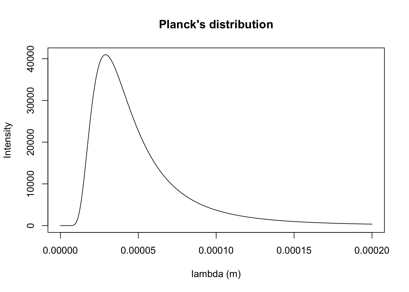
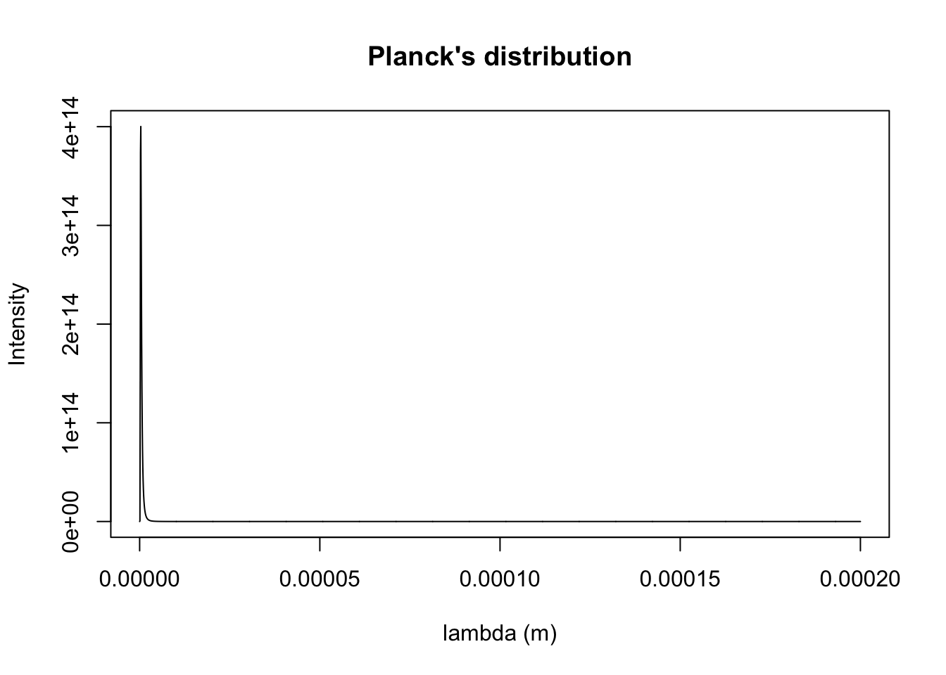
k1000 <- planck.distribution(x.min = 0.1e-9, x.max = 200000e-9, Temp = 1000, typ = "wavelength", plotQ = T)
k10000 <- planck.distribution(x.min = 0.1e-9, x.max = 200000e-9, Temp = 10000, typ = "wavelength", plotQ = T)